User manual

Datasets

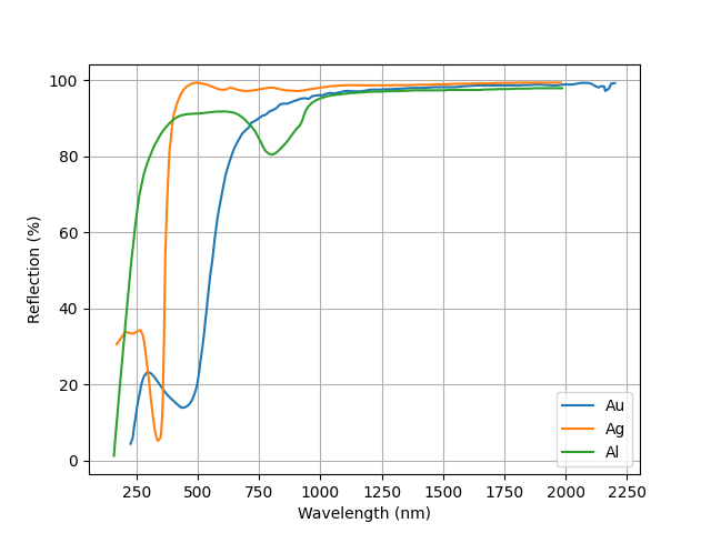
Mirror reflections data

The following code loads a wavelength-dependent reflection dataset of metal coated mirrors and plots a wavelength vs. reflection graph.

examples\example_EKSMA_OPTICS_mirrors.py

from scilightcon.datasets import load_EKSMA_OPTICS_mirror_reflections
import matplotlib.pyplot as plt

plt.figure()

for material in ['Au', 'Ag', 'Al']:
    data, headers = load_EKSMA_OPTICS_mirror_reflections(material)
    plt.plot(data[:,0], data[:,1], label = material)

plt.xlabel(headers[0])
plt.ylabel(headers[1])
plt.legend()
plt.grid()

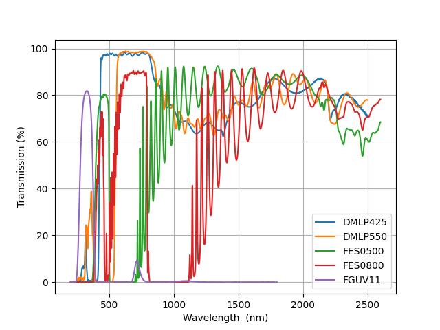
Transmission functions for Thorlabs filters

The following code loads a wavelength-dependent transmission dataset of Thorlabs filters and plots a wavelength vs. transmission graph. In this example only five filters are used.

load_THORLABS_filter_transmissions.py

from scilightcon.datasets import load_THORLABS_filter_transmissions
import matplotlib.pyplot as plt
import numpy as np

plt.figure()
plt.clf()

for material in ["DMLP425", "DMLP550", "FES0500", 'FES0800', "FGUV11"]:
    data, headers = load_THORLABS_filter_transmissions(material)

    x_values = data[:,0]
    y_values = data[:,1]
    filtered_x = [x_values[0]]
    filtered_y = [y_values[0]]
    h = [1/3, 1/3, 1/3]
    for x, y in zip(x_values, y_values):
        if not filtered_x or x>= filtered_x[-1]:
            filtered_x.append(x)
            filtered_y.append(y)
        else:
            pass

    y_values_smooth = np.convolve(filtered_y, h, 'same')
    y_values_smooth[-1] = (filtered_y[-1] + filtered_y[-2])/2
    y_values_smooth[-2] = (filtered_y[-1] + filtered_y[-2])/2
    y_values_smooth[0] = (y_values[0] + y_values[1])/2  
    y_values_smooth[1] = (y_values[0] + y_values[1])/2
    plt.plot(filtered_x, y_values_smooth, label = material)

plt.xlabel(headers[0])
plt.ylabel(headers[1])
plt.legend()
plt.grid()
plt.show()

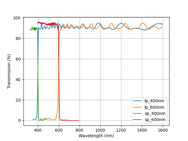
Transmission functions for Edmund Optics filters

The following code loads a wavelength-dependent transmission dataset for Edmund Optics filters and plots a wavelength vs. transmission graph. In this example only four filters are used.

load_EO_filter_transmissions.py

from scilightcon.datasets import load_EO_filter_transmissions
import matplotlib.pyplot as plt
import numpy as np

plt.figure()
plt.clf()

for material in ["lp_400nm", "lp_600nm", "sp_400nm", 'sp_600nm']:
    data, headers = load_EO_filter_transmissions(material)

    x_values = data[:,0]
    y_values = data[:,1]
    filtered_x = [x_values[0]]
    filtered_y = [y_values[0]]
    h = [1/3, 1/3, 1/3]
    for x, y in zip(x_values, y_values):
        if not filtered_x or x>= filtered_x[-1]:
            filtered_x.append(x)
            filtered_y.append(y)
        else:
            pass

    y_values_smooth = np.convolve(filtered_y, h, 'same')
    y_values_smooth[-1] = (filtered_y[-1] + filtered_y[-2])/2
    y_values_smooth[-2] = (filtered_y[-1] + filtered_y[-2])/2
    y_values_smooth[0] = (y_values[0] + y_values[1])/2  
    y_values_smooth[1] = (y_values[0] + y_values[1])/2
    plt.plot(filtered_x, y_values_smooth, label = material)

plt.xlabel(headers[0])
plt.ylabel(headers[1])
plt.legend()
plt.grid()
plt.show()

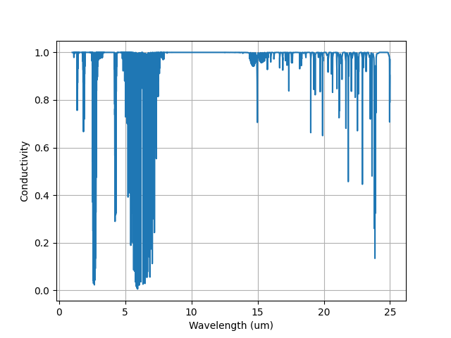
Atmospheric data

The following code loads an atmospheric dataset and plots a wavelength vs. conductivity graph.

load_atmospheric_data.py

from scilightcon.datasets import load_atmospheric_data
import matplotlib.pyplot as plt

plt.figure()
plt.clf()

data, headers = load_atmospheric_data()
data_file_name = 'atmosphere.csv'
plt.plot(data[:,0], data[:,1], label = material)

plt.xlabel(headers[0])
plt.ylabel(headers[1])
plt.grid()
plt.show()

Fitting

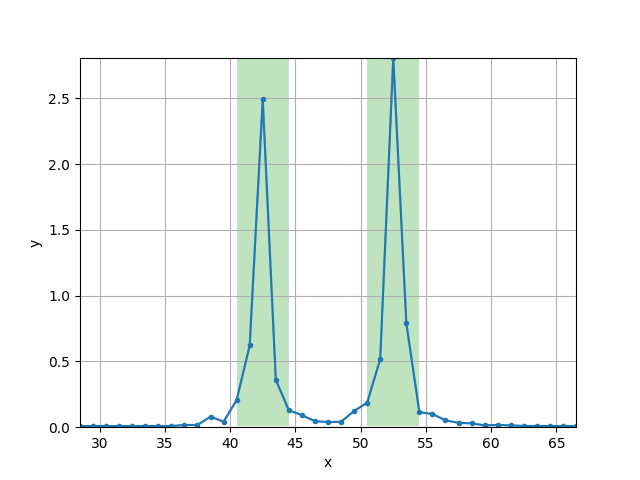
Peak detection

The following code is a peak detection function which can be used for several algorithms. In this case function prints out wavelengths at which the clusters that are above average. This is also represented in a graph.

examples\example_peak_detection.py

from scilightcon.fitting import detect_peaks
from scilightcon.datasets import load_csv_data
import matplotlib.pyplot as plt
import numpy as np

fname = 'data_test_detect_peaks.csv'

data, header = load_csv_data(fname)

x = data[:,0]
y = data[:,1]

method = "above_average"
clusters = detect_peaks(x, y, method = method, n_max=2)

plt.figure()

plt.plot(x, y, '.-')

print('clusters', clusters)
plt.plot(x, y, color='C0', alpha=0.3)
plt.xlim([x[0], x[-1]])

for cluster in clusters:
    plt.fill_between(x[cluster[0]:(cluster[1]+2)], np.min(y), np.max(y), facecolor = 'C2', alpha = 0.3)

plt.ylim([min([0.0, min(y)]), max(y)])

plt.xlabel("X")
plt.ylabel("Y")
plt.grid()

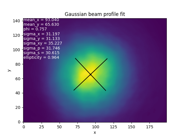
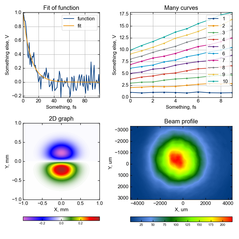
Laser beam profiling

Example of Gaussian fitting two-dimensional beam profile, loaded as two-dimensional variable matrix

examples\example_beam_profiler.py

from scilightcon.fitting import fit_beam_profile_2d
import matplotlib.pyplot as plt

results = fit_beam_profile_2d (matrix, method = 'gauss', options = {'decimation' : 2})

plt.figure()
plt.imshow(matrix, cmap='viridis', origin='lower')
plt.clim([0, None])
plt.xlabel('x')
plt.ylabel('y')
plt.title('Gaussian beam profile fit')

metrics = ['mean_x', 'mean_y', 'phi', 'sigma_x', 'sigma_y', 'sigma_xy', 'sigma_p', 'sigma_s', 'ellipticity']

plt.text(0, np.shape(matrix)[0], '\n'.join([f'{metric} = {result[metric]:.3f}' for metric in metrics]), fontdict={'color': 'white'}, va='top')
plt.plot(result['mean_x'], result['mean_y'], '.k')
plt.plot([result['mean_x'] - result['sigma_p'] * np.cos(result['phi']), result['mean_x'] + result['sigma_p'] * np.cos(result['phi'])],
    [result['mean_y'] - result['sigma_p'] * np.sin(result['phi']), result['mean_y'] + result['sigma_p'] * np.sin(result['phi'])],
    '-k')

plt.plot([result['mean_x'] - result['sigma_s'] * np.cos(result['phi']+np.pi/2.0), result['mean_x'] + result['sigma_s'] * np.cos(result['phi']+np.pi/2.0)],
    [result['mean_y'] - result['sigma_s'] * np.sin(result['phi']+np.pi/2.0), result['mean_y'] + result['sigma_s'] * np.sin(result['phi']+np.pi/2.0)],
    '-k')

Utilities

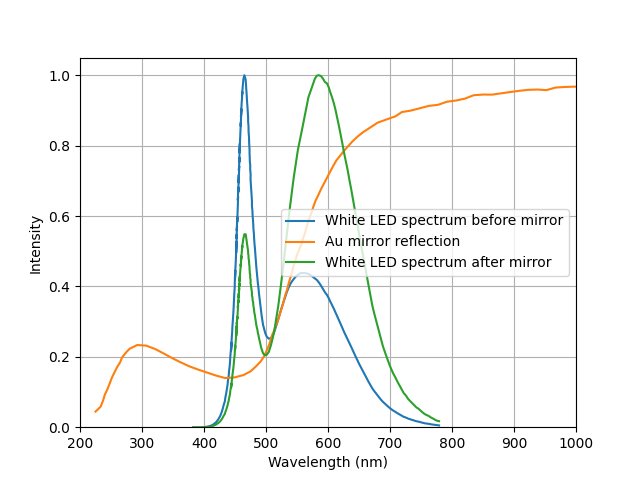
Multiplying several datasets with interpolation

The following code using interpolation and multiplication shows how white LED is reflected from gold coated mirror.

examples\example_interpolate_and_multiply.py

from scilightcon.datasets import load_csv_data
from scilightcon.datasets import load_EKSMA_OPTICS_mirror_reflections
from scilightcon.utils import interpolate_and_multiply
import matplotlib.pyplot as plt
import numpy as np

led_data, header = load_csv_data('White_LED_spectrum.csv')
led_x = led_data[:,0]
led_y = led_data[:,1]

mirror_data, headers = load_EKSMA_OPTICS_mirror_reflections('Au')
mirror_x = mirror_data[:,0]
mirror_y = mirror_data[:,1]

reflected_data = interpolate_and_multiply((led_x, led_y), (mirror_x, mirror_y))
reflected_x = reflected_data[0]
reflected_y = reflected_data[1]

plt.figure()

plt.plot(led_x, led_y/np.max(led_y), label = 'White LED spectrum before mirror')
plt.plot(mirror_x, mirror_y/np.max(mirror_y), label = 'Au mirror reflection')
plt.plot(reflected_x, reflected_y/np.max(reflected_y), label="White LED spectrum after mirror")

plt.xlabel(header[0])
plt.ylabel(header[1])
plt.xlim(200, 1000)
plt.ylim(0, None)
plt.legend()
plt.grid()

Logs reader

Collecting names of loggers

The following code collects and prints out a list of available loggers names in a given directory.

import datetime
from scilightcon.datasets import LogsReader

directory = r'\\konversija\kleja\ThermologgerLogs\v5'

reader = LogsReader(directory)
loggers_names_list = reader.list_loggers()

print(loggers_names_list)   

['Location 2B 314', 'Location 2D 3.14 Logger 1-4', 'Location 2D 3.14 Logger 5-8', 'Location 2D 3.14 Logger 9-12', 'Location 2D 3.14 Logger A', 'Location 2D 3.14 Logger B'...]

Collecting names of measurables

The following code collects and prints out a list of measurables names for a given logger name.

import datetime
from scilightcon.datasets import LogsReader

directory = r'\\konversija\kleja\ThermologgerLogs\v5'
logger_name = "Location 2B 314"

reader = LogsReader(directory)
measurables = reader.list_measurables(logger_name)

print(measurables)   

['A1-H Stalas 1', 'A1-H', 'A1-T Stalas 1', 'A1-T']

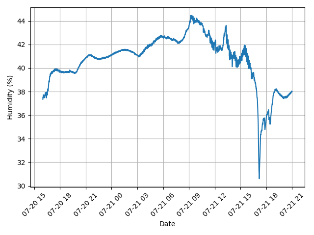
Retrieving data from the measurable

The following code checks if given logger_name and measurable are valid then collects timestamps and values for a given time period and displays them in a graph.

examples\example_logs_reader.py

import datetime
from scilightcon.datasets import LogsReader
import matplotlib.pyplot as plt

directory = r'\\konversija\kleja\ThermologgerLogs\v5'
logger_name = "Location 2B 314"
measurable="A1-H Stalas 1"

reader = LogsReader(directory)

loggers_names_list = reader.list_loggers()
print(loggers_names_list)                                       

measurables = reader.list_measurables(logger_name)
print (measurables)

from_date = datetime.datetime(2023,7,20, 16, 0, 0)
to_date = datetime.datetime(2023,7,21, 21, 0,0)
times, values = reader.get_data(
    logger_name=logger_name,
    measurable=measurable,
    from_date=from_date,
    to_date=to_date)

plt.plot_date(times, values, '-')
plt.grid()
cleaned_measurable = measurable.strip()
words_list = cleaned_measurable.split()
first_word = words_list[0]
if first_word[-1].upper() in ('T'):
    plt.ylabel("Temperature (°C)")
if first_word[-1].upper() in ('H'):
    plt.ylabel("Humidity (%)")
else:
    pass
plt.xlabel("Date")
plt.xticks(rotation=45)
plt.tight_layout()

Plotting

Default style

Light Conversion default style is loaded as matplotlib stylesheet with additional colormaps for drawing beam profiles (beam_profile), data (RdYlGnBu) or camera images (morgenstemning).

scilightcon styleDefault style

To enable the style, insert the following lines at the beginning of your script

from scilightcon.plot import apply_style

apply_style()

To reset the style to default:

from scilightcon.plot import reset_style()

reset_style()

Watermarks

To add one or multiple Light Conversion watermark(s), use scilightcon.plot.add_watermark() or scilightcon.plot.add_watermarks()

One watermarkMultiple watermarks

Call scilightcon.plot.add_watermark(plt.gcf()) at the end of the script.

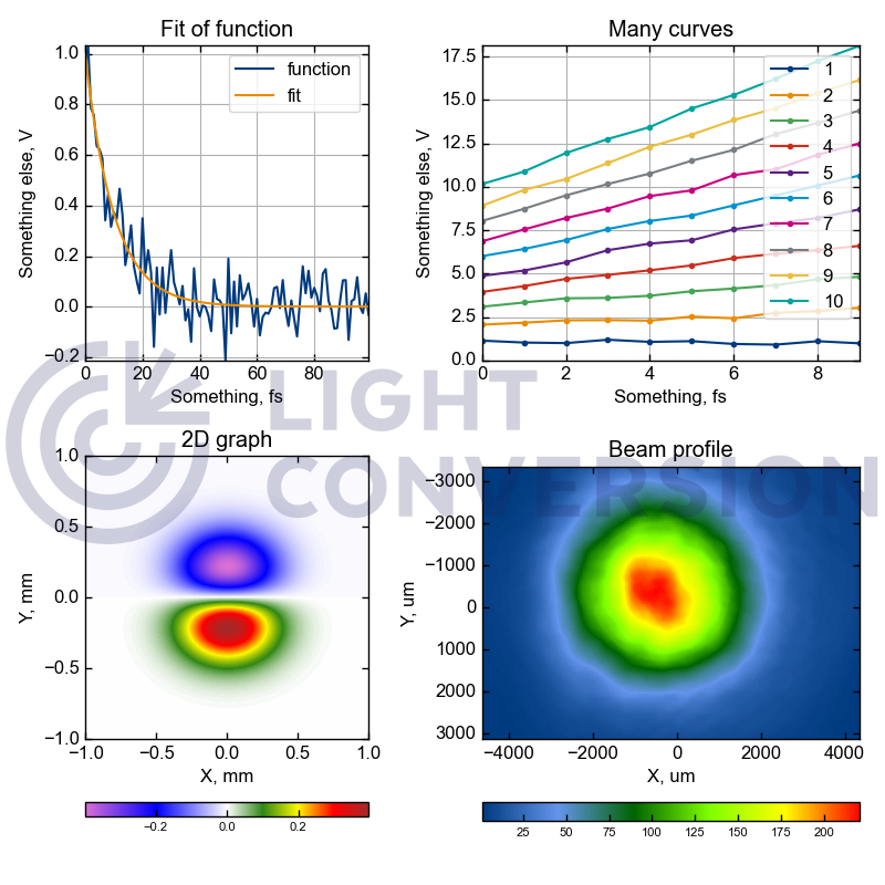
Call scilightcon.plot.add_watermarks(plt.gcf()) at the end of the script.